6. Data Analysis

First, let’s review what we have covered so far in the course, including simple Python variables, lists, dictionaries, functions, if statements, for loops, NumPy arrays, and descriptive statistics. Then, we will practice using these tools for data analysis.

6.1. Variables

Simple Python variables are used to hold individual data points. They can be modified using math operations and functions.

We can create simple variables with numbers, text, or boolean (True/False) data. All Python variables can be displayed using the print function.

integer = 4
decimal = 5.3
string = "Hello world."
tf = True
print(integer)
print(decimal)
print(string)
print(tf)

4
5.3
Hello world.
True

Each type of variable has ways we can operate on them. For numbers, we can do all the usual math operations.

a = 2
b = 3.5
c = 7
print(a * b)
print(a ** c)
print(a + b + c)

7.0
128
12.5

We can import the math module to get access to additional functions to do more advanced math operations and access mathmatical constants like \(\pi\) and \(e\).

import math
print(math.cos(2))
print(math.exp(1))
print(math.e ** 1)

-0.4161468365471424
2.718281828459045
2.718281828459045

There are also ways that we can work with text data. Strings can be concatenated (that is, combined) using the + operator.

s1 = "Hello"
s2 = "world."
print(s1 + " " + s2)

Hello world.

We can create strings from existing variables in various ways using f-strings.

user = "Mark S."
id_number = 634875
print(f"Greetings, {user} (id: {id_number})")

Greetings, Mark S. (id: 634875)

There are many functions for working with strings that we haven’t talked about much. We can see the functions that apply to a type of Python object using the help function.

# help(str)

For example, we can use startswith to check if a string starts with specific text, or endswith to check if it ends with some text.

s = "Hello world"
print(s.startswith("Hello"))
print(s.endswith("world"))

True
True

6.2. Lists

We can store sequences of any kind of variable in lists.

Lists always have square braces ([]) around them. Items are separated by commas. Lists are most helpful if there is some order to the data; for example, if we want to store the responses that a participant made in a series of trials in a psychology study. The trials occurred in a specific order, so a list is a natural way to store information about them.

numbers = [1, 2, 3]
letters = ["a", "b", "c"]
mix = [1, 2.3, "Hello world."]

Once we’ve placed created a list, we can add items onto the end using append. Sometimes, we may want to start with an empty list and add items to the end as needed; this can be useful together with for loops.

growing = []
growing.append(1)
growing.append(2)
growing.append(3)
print(growing)

[1, 2, 3]

We can access data in the list based on its position in the list. To get one item, we can use indexing. Similar to creating a list, we access parts of the list using square braces ([]).

Remember that, in Python, indexing starts at zero. This means that the first item in the list can be accessed using index 0.

trials = [1, 2, 3, 4, 5]
print(trials[0])
print(trials[4])

1
5

We can use negative indices also, to get items relative to the end of the list.

print(trials[-1])

5

We can also access part of a list to get a new list, using slicing. Slices are defined using start:stop syntax.

Slicing works to select the items in the list that are between the slice start and stop (see below).

list:  [  1,  2,  3,  4,  5  ]
index: [  0   1   2   3   4  ]
slice: [0   1   2   3   4   5]

If the start is not specified, then the slice will start at the beginning of the list. If the stop is not specified, then the slice will go until the end of the list.

print(trials[3:4])
print(trials[:2])
print(trials[3:])

[4]
[1, 2]
[4, 5]

We can use for loops to process data in lists and to create new lists. Here, we initialize an empty list, then loop over a list of numbers and calculate the square of each number, adding that onto the list of squares.

numbers = [1, 2, 3, 4]
squares = []
for n in numbers:
    squares.append(n ** 2)
print(squares)

[1, 4, 9, 16]

List comprehensions are a way to do this in one line of code, looping over items in a list and creating a new list from the old items.

squares2 = [n ** 2 for n in numbers]
print(squares2)

[1, 4, 9, 16]

6.3. Dictionaries

While lists are useful for storing sequences of data, Python dictionaries are useful for storing key, value pairs.

We can create a dictionary using curly braces ({}). Each key, value pair is indicated by a colon, and pairs are separated by commas. Keys can be most anything, but can’t be anything mutable, like lists, which can be changed after they are created.

For example, data for a study might be stored under a participant identifier key for the data for each participant.

d = {"001": 9, "002": 11, "003": 7}

The values of a dictionary can be any Python object. For example, this means we can have dictionaries of lists.

d2 = {"condition1": [1, 2, 3], "condition2": [4, 5, 6]}

We can even have dictionaries of dictionaries.

data = {
    "001": {"age": 23, "score": 9},
    "002": {"age": 29, "score": 11},
    "003": {"age": 32, "score": 10},
}

After creating a dictionary, we can continue adding key, value pairs using assignment. On the left side, we indicate a key that we want to define, then an equal sign and the value we want to assign to it. Note that we use square braces ([]) to access a dictionary, similarly to indexing a list, but we put in a key instead of a list index.

d3 = {"a": 1, "b": 2, "c": 3}
d3["d"] = 4
print(d3)

{'a': 1, 'b': 2, 'c': 3, 'd': 4}

We can access data in the dictionary using square braces also. We can use this to programmatically access data that has previously been stored in the dictionary.

print(data["001"])

{'age': 23, 'score': 9}

For example, we can write a function that will access data for any specified participant and display their information.

def print_summary(data, participant_id):
    age = data[participant_id]["age"]
    score = data[participant_id]["score"]
    print(f"{participant_id}: {age} years; score: {score}")

We can then use the function to access and display data for participants.

print_summary(data, "001")
print_summary(data, "002")

001: 23 years; score: 9
002: 29 years; score: 11

6.4. Functions

In addition to the built-in Python functions, we can easily create our own functions to complete repetitive tasks.

We define functions using the def keyword. Before writing a function, it’s a good idea to decide on what the inputs and outputs from the function should be. For example, say we want to make a function that squares numbers that are passed into that function. You should usually also include a one-line description at the start of the function as a docstring.

def square(x):
    """Calculate the square of a number."""
    return x ** 2

The list of inputs comes after the name of the function (square), within the parentheses (here, there is one variable called x). There is one output returned using the return statment (x ** 2).

We can also set default values. This can be very useful for more complex functions that can be configured in various ways. For example, the print function has a sep keyword that we can modify.

a = 1
b = 2
print(a, b)
print(a, b, sep=" ; ")

1 2
1 ; 2

We can define optional parameters to a function by adding an equal sign and some default value after a function input. This lets us set some default value that can be modified when calling the function.

def power(x, pow=2):
    """Calculate some power of a number."""
    return x ** pow
print(power(2))
print(power(2, pow=8))

4
256

6.5. If/elif/else statements

We can use tests of conditions to determine what code to run. They are often useful in combination with functions, allowing a function to change what it runs depending on the inputs that are passed to it.

The simplest way to use an if statement is by checking one condition.

def greeting(user):
    """Print a greeting to a user."""
    if user == "world":
        print("Hello world.")
greeting("world")
greeting("someone else")  # doesn't print anything

Hello world.

We can also use more complex if statements to check for multiple conditions. For example, say we want to make a function that can calculate various statistics. We can use multiple if/elif statements to check for a series of different conditions. The conditions are checked in order, and the first one that is True is run. If the stat is "mean", then the return np.mean(x) line will run. If the stat is "std", then the first two checks will be False, and then the third block will run return np.std(x).

import numpy as np
y = np.array([3, 9, 3, 4, 1, 7, 8, 5, 4])
def calculate_stat(x, stat):
    """Calculate a statistic from a set of observations."""
    if stat == "mean":
        return np.mean(x)
    elif stat == "median":
        return np.median(x)
    elif stat == "std":
        return np.std(x)
    else:
        raise ValueError(f"Unknown statistic: {stat}")
print(calculate_stat(y, "mean"))
print(calculate_stat(y, "std"))
# calculate_stat(y, "min")  # throws an error because we the calculate_stat function doesn't expect it

4.888888888888889
2.469567863432541

When we are checking for multiple conditions, it’s a good idea to include an else statement that runs in case none of the conditions applied. In that case, we can’t really run the function, so we’ll raise an exception. In this case, we use a ValueError, which indicates that we encountered an unexpected value in the function inputs.

6.6. For loops

Sometimes, we may want to run some code multiple times, such as running the same operation on each item in a list. We can do this using for loops.

Say we have a list indicating the condition code for a set of trials in a psychology study, and we want to count up the number of trials for each condition. Here, each trial is either a “target” trial or a “lure” trial.

trial_type = ["target", "target", "lure", "target", "lure", "target", "target", "lure"]

For example, we can use a for loop with a counter to get the number of target trials. The += operator takes a variable (in this case, count) and adds a number to it. For example, count += 1 adds 1 to the current value of count.

count = 0
for tt in trial_type:
    if tt == "target":
        count += 1
print(count)

5

This code is a lot easier to use if we put it in a function. Let’s define a function that can work on any list of trial type codes. We’ll take in two inputs, which indicate the trial labels indicating their type, and the type that we want to count. We’ll have the default to “target”. The function will return the number of times that the type_to_count appears in the list of trials.

def count_trials(trial_types, type_to_count="target"):
    """Count the number of trials matching a type."""
    count = 0
    for tt in trial_types:
        if tt == type_to_count:
            count += 1
    return count

Now we have a function that can count any trial types we want.

trial_type = ["target", "target", "lure", "target", "lure", "target", "target", "lure"]
lure_count = count_trials(trial_type, type_to_count="lure")
print(lure_count)

3

We can also loop over multiple lists at the same time using the zip function. For example, say we have trial type and response on each of a set of trials.

trial_type = ["target", "lure", "lure", "target", "lure", "target", "target", "lure"]
response = ["old", "old", "new", "old", "new", "new", "old", "new"]

This code will count the number of responses that are hits and false alarms.

hits = 0
false_alarms = 0
for tt, r in zip(trial_type, response):
    if tt == "target" and r == "old":
        hits += 1
    elif tt == "lure" and r == "old":
        false_alarms += 1
print(hits, false_alarms)

3 1

For problems like this, it’s convenient to loop over both lists at the same time using zip. Note that we need to unpack the two outputs of zip on each part of the loop. The tt variable gets the current trial type, while the r variable gets the current response.

6.7. NumPy arrays

While we can organize data in lists in Python, for many scientific applications it’s easier to work with NumPy arrays instead. Arrays are designed for working with sets of data points, such as response accuracy or response times on individual trials.

For example, say that we have a series of labels for trials in a study, indicating whether the response was correct (coded as 1) or incorrect (coded as 0). We can use an array to hold this information for each trial.

correct = np.array([0, 1, 0, 0, 0, 1, 1, 1, 0, 1, 1, 1])
print(correct)

[0 1 0 0 0 1 1 1 0 1 1 1]

We can use NumPy functions to calculate various statistics, such as the sum (which here corresponds to the total number of correct responses) and the mean (which here corresponds to the fraction correct).

total = np.sum(correct)
n = correct.size
accuracy = np.mean(correct)
print(f"{total} correct out of {n}; {round(accuracy * 100)}% accuracy")

7 correct out of 12; 58% accuracy

If we want to get information about some subset of trials, we can use slicing to access data based on its position in the array. For example, using slicing, we can split the trials in half and calculate accuracy for the first and second halves.

accuracy1 = np.mean(correct[:6])
accuracy2 = np.mean(correct[6:])
print(f"Half 1: {round(accuracy1 * 100)}% accuracy")
print(f"Half 2: {round(accuracy2 * 100)}% accuracy")

Half 1: 33% accuracy
Half 2: 83% accuracy

We can also use indexing to access individual trials. In this case, we will get an integer instead of an array.

is5corr = correct[4]  # index 4 corresponds to trial number 5
print(is5corr)
print(type(is5corr))

0
<class 'numpy.int64'>

There are various functions to generate special types of arrays, such as arrays with all ones or all zeros, in a specified shape.

a = np.ones(4)
b = np.zeros((4, 5))
print(a)
print(b)

[1. 1. 1. 1.]
[[0. 0. 0. 0. 0.]
 [0. 0. 0. 0. 0.]
 [0. 0. 0. 0. 0.]
 [0. 0. 0. 0. 0.]]

Other functions can generate a range of values. The arange function can generate values between a start value and a stop value, with a specific step size. The default step size is one.

r1 = np.arange(1, 11)
r2 = np.arange(1, 11, 2)
print(r1)
print(r2)

[ 1  2  3  4  5  6  7  8  9 10]
[1 3 5 7 9]

If only one value is given, then the range will be from 0 to that number.

r3 = np.arange(11)
print(r3)

[ 0  1  2  3  4  5  6  7  8  9 10]

The linspace function also generates values within an interval, but instead of a step size, you indicate the number of samples you want.

l1 = np.linspace(0, 10, 5)
l2 = np.linspace(0, 10, 11)
print(l1)
print(l2)

[ 0.   2.5  5.   7.5 10. ]
[ 0.  1.  2.  3.  4.  5.  6.  7.  8.  9. 10.]

We can use comparison operators (==, !=, >, <, >=, <=) to create boolean arrays, which can then be used to filter arrays with the same shape. We can also combine comparisons using these operators: not (~), and (&), or (|).

For example, say we have the following arrays defining trial type and response.

trial_type = np.array(["target", "lure", "lure", "target", "lure", "target", "target", "lure"])
response = np.array(["old", "old", "new", "old", "new", "new", "old", "new"])

We can get just trials that were hits by combining a check for a “target” trial and an “old” response.

is_hit = (trial_type == "target") & (response == "old")

We can use a boolean array with np.sum to measure the number of trials matching that filter.

n_hit = np.sum(is_hit)
print(n_hit)

3

We can also use it to filter another array with the same shape. For example, say we have another array with response times in seconds. We can use the is_hit filter to get response times for just the hit responses.

response_time = np.array([5.4, 3.4, 8.4, 3.2, 3.9, 5.2, 6.1, 7.1])
response_time[is_hit]

array([5.4, 3.2, 6.1])

We can put these things together to calculate mean response time for hits, in one line of code.

hit_rt = np.mean(response_time[(trial_type == "target") & (response == "old")])
print(hit_rt)

4.9

Array dimensions make it possible to organize data based on how it varies according to different measurements. For example, we can use a 1D array to represent a sequence of trials that we want to analyze.

response_time_trials = np.array([1.2, 2.3, 1.4, 1.8])

We can use other dimensions to organize data also. For example, a common approach is to have one dimension indicate the results of different trials or tests, and another dimension that indicates the participant that was tested. To create an array with two dimensions, we can use a list of lists. Each list becomes a row in the 2D array (also known as a matrix).

test_scores = np.array(
    [[7, 8, 3, 4],
     [4, 7, 2, 5],
     [5, 9, 3, 3]]
)

For example, this array indicates that the first subject got scores of 7, 8, 3, and 4 on the different tests. The second test had higher scores than the other tests, with the three subjects scoring 8, 7, and 9.

If we want to look up the score for one subject and test, we can do that using indexing. For example, here we get the score for the second participant and first test.

test_scores[1, 0]

np.int64(4)

We can also use slicing to get a range of data. For example, we can get the first two scores or the last two scores.

print(test_scores[:, :2])  # get the first two tests
print(test_scores[:, 2:])  # get the last two tests

[[7 8]
 [4 7]
 [5 9]]
[[3 4]
 [2 5]
 [3 3]]

When we have multiple dimensions, we can analyze those dimensions separately by setting the axis argument in NumPy functions. With no axis argument, NumPy operates on all elements, regardless of dimension. Here, using np.mean with the default arguments gives the average score, averaged across subjects and tests.

np.mean(test_scores)

np.float64(5.0)

Setting axis=0 calculates an average across rows, separately for each column. In this example, that lets us calculate the average score for each test, averaged across subjects. We can see that the average score was highest on the second test.

np.mean(test_scores, axis=0)

array([5.33333333, 8.        , 2.66666667, 4.        ])

Setting axis=1 calculates an average across columns, separately for each column. In this example, that lets us calculate the average score for each subject, averaged across tests. We can see that the first subject had the highest average score.

np.mean(test_scores, axis=1)

array([5.5, 4.5, 5. ])

6.8. Descriptive statistics

When we have a series of observations, we can use descriptive statistics to summarize those observations by measuring central tendency and spread.

For example, say we have measured a series of response times.

response_times = np.array(
    [2.2, 2.8, 3.4, 6.2, 3.7, 5.5, 3.9, 4.2, 4.5, 5.1, 5.8, 3.2, 2.8, 2.9, 3.0, 3.1, 4.2, 2.8, 2.9, 3.7, 3.5, 6.7, 3.8, 4.8, 2.3]
)

We can use a histogram to get a view of the overall distribution.

import matplotlib.pyplot as plt
values, bins, bars = plt.hist(response_times)

We can measure central tendency using the mean (the sum of all values divided by the number of samples) or the median (the center value after ranking values).

values, bins, bars = plt.hist(response_times)
h1 = plt.vlines(np.median(response_times), 0, 6, color="red")
h2 = plt.vlines(np.mean(response_times), 0, 6, color="purple")
plt.legend([h1, h2], ["median", "mean"]);

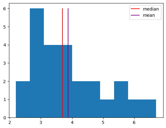
We can measure the spread of a distribution using the range (the difference the minimum value and the maximum value) or the standard deviation (essentially the average distance of samples from the mean).

sd = np.std(response_times)
r = np.max(response_times) - np.min(response_times)
print(f"Standard deviation: {sd:.1f}; range: {r}")

Standard deviation: 1.2; range: 4.5

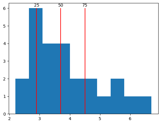
We can also get percentiles of the distribution to better understand how the observations vary. A percentile \(p\) indicates the value where \(p\) percent of samples are less than that value.

qs = [25, 50, 75]
ps = np.percentile(response_times, qs)
values, bins, bars = plt.hist(response_times)
plt.vlines(ps, 0, 6, color="red")
for q, p in zip(qs, ps):
    plt.text(p, 6.1, f"{q}", ha="center")

In NumPy arrays, the special value NaN (not-a-number) indicates when data for some observation is missing. For example, say that a participant was asked to make a response on each of 10 trials, but did not make a response on two of the trials. In that case, we would not have a measure of response time on those trials.

rt_missing = np.array([3.4, np.nan, 4.2, 5.3, 2.5, np.nan, 5.2, 5.9, 3.2, 4.7])

If we use normal NumPy functions, we will often get NaN, because many statistics are undefined if a sample is missing.

print(np.mean(rt_missing))
print(np.std(rt_missing))

nan
nan

However, we can use special functions with nan at the start that omit missing samples and calculate a statistic using the available samples.

print(np.nanmean(rt_missing))
print(np.nanmedian(rt_missing))
print(np.nanstd(rt_missing))

4.3
4.45
1.1067971810589328

We cannot check for NaN values using standard comparison operators like ==.

rt_missing == np.nan

array([False, False, False, False, False, False, False, False, False,
       False])

Nothing is equal to NaN, not even NaN, so comparison doesn’t work the usual way.

Instead, we can use np.isnan to check for missing values.

np.isnan(rt_missing)

array([False,  True, False, False, False,  True, False, False, False,
       False])

We can combine np.isnan with np.sum to get the number of missing observations.

np.sum(np.isnan(rt_missing))

np.int64(2)

To get only defined observations, we can filter to get non-NaN items.

rt_clean = rt_missing[~np.isnan(rt_missing)]
rt_clean

array([3.4, 4.2, 5.3, 2.5, 5.2, 5.9, 3.2, 4.7])

6.9. Saving and loading data

Scientific observations are generally saved in data files that can be stored for later analysis. Utilties to save and load data faciliate this process.

Data stored in a NumPy array can be saved to a file using np.savetxt, which stores data in a human-readable format, or np.save, which stores data in a NumPy format that is more compact, more precise, and faster to read and write but is not human readable.

np.savetxt("data/response_time.txt", response_time)
np.save("data/response_time.npy", response_time)

We can load data from a file into a NumPy array using np.loadtxt (if the file is in text format) or np.load (if the file is in NumPy format).

rt1 = np.loadtxt("data/response_time.txt")
rt2 = np.load("data/response_time.npy")
print(rt1)
print(rt2)

[5.4 3.4 8.4 3.2 3.9 5.2 6.1 7.1]
[5.4 3.4 8.4 3.2 3.9 5.2 6.1 7.1]

If we have multiple arrays that we want to save to a file, we can use np.savez. Note that, when saving multiple arrays, we must give each array a name. Here, we’ll give each array the same name as the corresponding variable.

np.savez(
    "data/trials.npz", 
    trial_type=trial_type, 
    response=response,
    response_time=response_time,
)

When using np.load with an .npz file, we will get a dictionary-like object that lets us access each of the arrays that were saved to the file.

arrays = np.load("data/trials.npz")
arrays["trial_type"]

array(['target', 'lure', 'lure', 'target', 'lure', 'target', 'target',
       'lure'], dtype='<U6')

6.10. Data analysis

When analyzing data, we can use any of the programming tools we have learned so far.

As an example, we will analyze simulated data from a hypothetical recognition memory study. In this study, participants studied items (either words or pictures) to try to remember them for a later memory test. During the test, participants were shown target items that they studied previously and lure items that they had not previously seen. Their task was to view each item and respond old if they think they saw it before, or new if they think they did not see it before.

Data are split into one .npz file for each participant. Each file has arrays indicating subject, trial, study_time (length of exposure to each studied item in seconds), item_type (word or picture), trial_type (target or lure), and response (1 for old or 0 for new) for each trial. For target trials, an “old” response (coded as 1) is correct. For lure trials, a “new” response (coded as 0) is correct.

We can load data from one subject using np.load. In this case, because our data include strings, we must set allow_pickle=True.

data = np.load("data/sub-01_beh.npz", allow_pickle=True)

We can get the names of the variables in the file using the keys method. We convert the result to a list for easier viewing.

list(data.keys())

['subject', 'trial', 'study_time', 'item_type', 'trial_type', 'response']

For example, we can access the trial_type key to get an array with the trial type (target or lure) for each trial for this subject. To see a subset of the array, we can use array slicing.

data["trial_type"][8:12]

array(['target', 'target', 'lure', 'lure'], dtype=object)

Exercise: calculating memory performance

Calculate the hit rate and false alarm rate for subject 01, whose data are read into the response and trial_type variables below. Hit rate is defined as the fraction of target trials where the participant responded “old” (here, coded as 1 in the response variable). False-alarm rate is defined as the fraction of lure trials where the participant responded “new” (here, coded as 0 in the response variable). The type of each trial (target or lure) is indicated in the trial_type variable.

If the (simulated) participant was able to remember the studied material, then their hit rate should be greater than the false alarm rate. Does it seem like they were able to remember the material?

response = data["response"]
trial_type = data["trial_type"]

# answer here

Exercise: comparing item types

Calculate the hit rate for subject 01, separately for word and picture trials. Hit rate is defined as the fraction of target trials where the participant responded “old” (here, coded as 1 in the response variable). Item type is indicated in the item_type variable (word or picture).

Was the hit rate different for words and pictures? Which type of stimulus seems like it was better remembered?

item_type = data["item_type"]

# answer here

Exercise: writing an analysis function

Write a function that takes arrays with the trial type (target or lure) and response (1 for “old”, 0 for “new”) and returns the hit rate. Write a one-line docstring indicating what your function does. Add an optional parameter to your function to let you either calculate hit rate or corrected hit rate, which is the hit rate minus the false-alarm rate.

Test your function by using it to calculate hit rate and corrected hit rate for subject 01.

# answer here

Exercise: analyzing data from multiple subjects

Use your function to calculate the corrected hit rate for subjects 01 through 08 (the identifiers are in the list defined below) and append it to the corrected_hr list (initialized below). The data for each subject are in data/sub-XX_beh.npz.

What is the mean corrected hit rate across subjects? What is the standard deviation? Does it seem like most subjects were able to remember the stimuli?

subjects = ["01", "02", "03", "04", "05", "06", "07", "08"]
corrected_hr = []

# answer here

6.11. Summary

We can represent data using various data structures, depending on which is the best fit for what we are trying to do. After representing the data, we can use programming tools and analysis functions to conduct analyses.

We can use lists to represent sequences of data, such as information about a sequence of trials in a study. If we want to be able to analyze a set of observations as a whole (for example, to calculate descriptive statistics such as the mean or standard deviation), NumPy arrays are more suitable than lists.

To represent information about different variables in one data structure, we can use dictionaries. NumPy uses dictionary-like objects to represent multiple arrays within a file.

To carry out the same analysis on multiple subsets of data, we can define a function to perform the analysis using def and return. Using if statements allows us to make functions more flexible. We can analyze data from multiple subjects using for loops.