Scientific computing in Python#
While the base Python language can be used for scientific applications, most scientific work in Python uses the NumPy (Numeric Python) package to work with arrays of datapoints.
Limitations of basic Python#
We can do a lot with the basic Python data structures, like lists and dictionaries. But for handling scientific data, like responses in a psychology study, they aren’t very easy to work with.
For example, say that a participant in a study was shown a list of words, and then shown another list of words and asked to say whether each one was shown before (old) or not (new). On each trial, we have two pieces of information to keep track of: whether it was a target or a lure, and whether they said it was old or new. We can put this information into two Python lists.
trial_type = ["target", "lure", "lure", "target", "lure", "target", "target", "lure"]
response = ["old", "old", "new", "old", "new", "new", "old", "new"]
Using a for loop and an if/elif statement, we can then score the responses to get the number of hits and false alarms.
hits = 0
false_alarms = 0
for tt, r in zip(trial_type, response):
    if tt == "target" and r == "old":
        hits += 1
    elif tt == "lure" and r == "old":
        false_alarms += 1
Finally, we can calculate hit rate (HR) and false alarm rate (FAR) by counting the number of trials in each condition and dividing by that.
n_targets = 0
n_lures = 0
for tt in trial_type:
    if tt == "target":
        n_targets += 1
    else:
        n_lures += 1
hr = hits / n_targets
far = false_alarms / n_lures
print(f"Hit rate: {hr}, false alarm rate: {far}")
Hit rate: 0.75, false alarm rate: 0.25
As we can see from the example, it’s possible to analyze scientific data using Python lists. But it took multiple for loops and if statements. And it will run pretty slowly, if you have a lot of data. Fortunately, there’s a better way.
NumPy arrays#
In science, we often have arrays of data, corresponding to multiple measurements of some variable. To analyze the data, we may need to sort these measurements into different conditions and calculate various statistics. NumPy (Numeric Python) is designed to make this process easier using a new data type called ndarray, or N-dimensional array.
First, we need to make sure NumPy is installed. It is not a built-in Python package, so we must install it from the Python Package Index (PyPI). If you have set up the datascipsych project, you should already have it set up in your environment. See the README for installation instructions.
If NumPy is installed, you should be able to import it. We will use the conventional way of importing NumPy, using import numpy as np. NumPy functions can then be called using np.[function_name].
import numpy as np
from IPython.display import display
NumPy lets us put multiple measurements of the same type into an array that is designed for data analysis. We can do this by calling np.array and passing in a list of data.
integers = np.array([1, 2, 3])
floats = np.array([1.1, 2.2, 3.3])
letters = np.array(["a", "b", "c"])
print(integers, floats, letters)
[1 2 3] [1.1 2.2 3.3] ['a' 'b' 'c']
Each array has one datatype, indicating the type of data stored in it.
print(integers.dtype, floats.dtype, letters.dtype)
int64 float64 <U1
The integers are stored as 64-bit integers, the decimals as 64-bit floats, and the letters as strings (the “U” stands for unicode, a common data format for representing text). NumPy automatically uses the smallest length of string possible to hold the data, so it stores our one-character strings using one character (U1) for each part of the array.
Each array also has a size attribute that tells total size (i.e., the number of elements) of the array. The ndim attribute tells us how many dimensions an array has. So far, we’re just using 1-dimensional arrays. The shape attribute gives the size of each dimension.
print(f"Total size of the array: {integers.size}")
print(f"Number of dimensions: {integers.ndim}")
print(f"Size of each dimension: {integers.shape}")
Total size of the array: 3
Number of dimensions: 1
Size of each dimension: (3,)
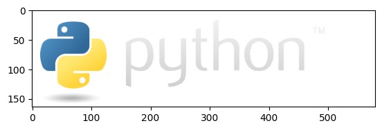
We can also make arrays with multiple dimensions. For example, if we read in a PNG image, we will have three dimensions: height, width, and color/transparency. Here, we’ll use the Matplotlib library to read a PNG file into a NumPy array. We’ll also plot it so we can see what the image is.
import matplotlib.pyplot as plt
image = plt.imread('python-logo.png')
print(f"Dimensions: {image.ndim}, Shape: {image.shape}")
ax = plt.imshow(image)
Dimensions: 3, Shape: (164, 580, 4)
We will mostly work with 1D arrays. But NumPy can handle any number of dimensions, which can be very helpful for working with more complex data.
Exercise: NumPy arrays#
Create an array called a with these integers: 4, 3, 2, 1
Create an array called b with these floats: 1.4, 2.3, 1.9
Use array attributes to get the size, number of dimensions, and shape of your b array.
# answer here
Array expressions#
When data are in an array, we can work with whole arrays together as a unit. For example, we can operate on a whole array using math expressions.
floats = np.array([1.1, 2.2, 3.3])
print(floats + 2)
print(floats * 2)
print(floats ** 2)
[3.1 4.2 5.3]
[2.2 4.4 6.6]
[ 1.21  4.84 10.89]
Notice that this is a lot easier using NumPy arrays than it would be using lists. We could use list comprehensions to do something similar, but it’s harder to read and slower to run.
f_list = [1.1, 2.2, 3.3]
print([f + 2 for f in f_list])
print([f * 2 for f in f_list])
print([f ** 2 for f in f_list])
[3.1, 4.2, 5.3]
[2.2, 4.4, 6.6]
[1.2100000000000002, 4.840000000000001, 10.889999999999999]
Using NumPy arrays, we can also use operations to make calculations with whole arrays.
integers = np.array([1, 2, 3])
floats = np.array([1.1, 2.2, 3.3])
print(integers + floats)
print(integers * floats)
[2.1 4.2 6.3]
[1.1 4.4 9.9]
Note that the operations we just saw are all elementwise. That is, we are not using matrix multiplication. Instead, we’re just taking each element of each array and adding them or multiplying them together.
We can calculate matrix multiplication also, using the @ operator. For example, we can calculate the dot product of our floats vector. (Don’t worry about this if you don’t know about matrix multiplication.)
print(floats @ floats)
16.939999999999998
Exercise: array expressions#
Create an array x with the numbers 1, 2, 3, and 4. Calculate x * 2 and x ** 2. Create another array y with numbers 5, 6, 7, and 8. Calculate x + y.
Advanced#
Calculate the dot product between x and y. This is the sum of the product of each element of x and y. You can calculate it using matrix multiplication.
# answer here
Creating arrays#
We can create arrays in two basic ways. First, as we’ve seen, we can create a list and convert (or cast) it into an array.
a = np.array([6, 5, 4, 3, 2, 1])
a
array([6, 5, 4, 3, 2, 1])
We can also use various NumPy functions to make arrays of specific shapes. For example, we can create an array with all zeros using np.zeros.
z = np.zeros(6, dtype=int)
z
array([0, 0, 0, 0, 0, 0])
The optional dtype argument lets us set the data type of the array. For example, we can use this with np.zeros to create a boolean array that is False at each position in the array.
all_false = np.zeros(5, dtype=bool)
all_false
array([False, False, False, False, False])
Boolean arrays are sometimes used to filter other arrays. For example, say we have one array with data, and another array determining whether each data point should be included.
data = np.array([10.2, 15.4, 13.1, 15.0])
include = np.array([True, True, False, True])
data[include]
array([10.2, 15.4, 15. ])
We can index an array with a boolean array, and get back just the items where the boolean array is True. We will talk more about array filtering later.
NumPy has functions to make two common types of arrays, filled with all zeros (as we just saw) or all ones.
np.zeros(4)
array([0., 0., 0., 0.])
The shape argument can take an integer, if there is just one dimension, or a tuple, if there are multiple dimensions. Here, we’ll create an array with 5 rows and 2 columns.
np.ones((5, 2))
array([[1., 1.],
       [1., 1.],
       [1., 1.],
       [1., 1.],
       [1., 1.]])
It’s also often useful to make an array with numbers in order. We can do this using np.arange. The end-point is non-inclusive; for example, if we pass 6, then the last item will be 5. This is similar to how indexing works; by default, np.arange starts counting at 0.
np.arange(6)
array([0, 1, 2, 3, 4, 5])
We can adjust the starting and stopping point of the array. If we pass two arguments, the first will be the starting point, and the last will be the ending point.
np.arange(1, 11)
array([ 1, 2, 3, 4, 5, 6, 7, 8, 9, 10])
Note that the upper bound is non-inclusive.
Finally, we can make increasing values in a more flexible way using np.linspace.
np.linspace(0, 1, 11)
array([0. , 0.1, 0.2, 0.3, 0.4, 0.5, 0.6, 0.7, 0.8, 0.9, 1. ])
Here, we make 11 values ranging from 0 to 1, with the values being evenly spaced.
Exercise: creating arrays#
Use the np.ones function to create an array called a with 6 ones.
Use the np.zeros function to create a 2 x 2 array called b with zeros.
Use the np.arange function to create an array called c with the numbers 1 through 5.
# answer here
Accessing data in arrays#
Just like we saw before with lists, we can access data in an array using indexing and slicing.
a = np.arange(1, 11)
a
array([ 1, 2, 3, 4, 5, 6, 7, 8, 9, 10])
print(a[9])
10
a[:5]
array([1, 2, 3, 4, 5])
Things get a little more complicated for 2D arrays, because we can specify indexes for both dimensions. First, let’s make a matrix by passing in a list of lists to np.array.
matrix = np.array([[1, 2, 3], [4, 5, 6], [7, 8, 9]])
matrix
array([[1, 2, 3],
       [4, 5, 6],
       [7, 8, 9]])
We can access part of the matrix using indexing, if we pass indexes for both dimensions. This will get number at the second row and third column.
print(matrix[1, 2])
6
We can take slices through either dimension, or both, to access data from part of the matrix. Here, we’ll get the first two rows and last two columns.
matrix[:2, 1:]
array([[2, 3],
       [5, 6]])
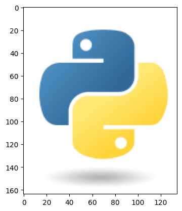
For example, let’s look again at the PNG image we loaded before. We’ll reload it here to make sure we have it in memory. We can use slicing to crop the image by getting the first 135 columns, so that we just have the Python logo without the text.
image = plt.imread('python-logo.png')
ax = plt.imshow(image[:, :135])
When we take a slice of an array, we get what NumPy calls a view of the array. Instead of making a new array with the data in the part that we accessed, we get a “view” of that part of the array. This means that, if we change the data in our “view”, we modify the original array.
a = np.arange(1, 11)
b = a[:5]
b += 10
a
array([11, 12, 13, 14, 15, 6, 7, 8, 9, 10])
If we want to copy the sub-array instead, we can use the copy method.
a = np.arange(1, 11)
b = a[:5].copy()
b += 10
a
array([ 1, 2, 3, 4, 5, 6, 7, 8, 9, 10])
Note that, this time, the original a array isn’t affected when we change b. This is because b is now a copy of a instead of a view.
Exercise: accessing data in arrays#
Create an array a with the numbers 1:10. Print the third element in the array. Then use slicing to get a view of the array b that includes the numbers 4-6.
# answer here
Array functions#
We can use various functions to work with data in NumPy arrays.
The np.sum function calculates the total for an array.
correct = np.array([0, 1, 1, 0, 0, 0, 1, 0, 1, 1, 1, 1])
total = np.sum(correct)
print(f"Total correct: {total}")
Total correct: 7
The np.mean function can be used to calculate the mean of an array (that is, the sum divided by the number of observations). If we have an array with 1 for correct and 0 for incorrect, we can use the mean to calculate accuracy as the fraction of correct responses.
accuracy = np.mean(correct)
print(f"Accuracy: {round(accuracy * 100)}%")
Accuracy: 58%
Exercise: array functions#
Say that a study participant completed eight trials of a memory task. They answered correctly on trials 1, 2, 4, 5, and 8, and answered incorrectly on the other trials.
Define an array called correct with 1 on correct trials and 0 on incorrect trials. Calculate the overall accuracy (that is, the fraction of correct trials).
Advanced#
Print out the accuracy as a percentage.
# answer here
Filtering arrays#
We can use boolean arrays to quickly filter arrays.
We can index a NumPy array using another array. This lets us quickly get different subsets of data. For example, say we measured response time in two different conditions, labeled condition 1 and condition 2.
response_time = np.array([1.2, 3.5, 1.4, 2.7, 1.8, 4.1, 1.7, 4.5])
condition = np.array([1, 2, 1, 2, 1, 2, 1, 2])
To filter the response_time array, we first create a boolean array.
condition == 1
array([ True, False, True, False, True, False, True, False])
We can use this array to index the response_time array and get must the observations for that condition.
response_time[condition == 1]
array([1.2, 1.4, 1.8, 1.7])
Finally, we can use np.mean to calculate the mean response time for condition 1 and condition 2.
rt1 = np.mean(response_time[condition == 1])
rt2 = np.mean(response_time[condition == 2])
print(f"Mean RT (condition 1): {rt1}")
print(f"Mean RT (condition 2): {rt2}")
Mean RT (condition 1): 1.525
Mean RT (condition 2): 3.7
Similar to how we can combine conditionals with the and, or, and not keywords, we can do something similar with arrays. However, we need to use different symbols when working with arrays.
To negate an array, we use ~ instead of not. Note that we need to add parentheses around the statement (condition == 1) to use this here.
print(condition == 1)
print(~(condition == 1))
[ True False  True False  True False  True False]
[False  True False  True False  True False  True]
To combine two conditionals, we can use & instead of and. Note how the output is only True when both conditionals apply.
print(response_time < 3)
print(condition == 2)
print((response_time < 3) & (condition == 2))
[ True False  True  True  True False  True False]
[False  True False  True False  True False  True]
[False False False  True False False False False]
We can also use | instead of or.
print(response_time < 1.5)
print(condition == 2)
print((response_time < 1.5) | (condition == 2))
[ True False  True False False False False False]
[False  True False  True False  True False  True]
[ True  True  True  True False  True False  True]
Make sure to put parentheses around each conditional statement that you are combining. If you leave out the parentheses, it may change the order of operations in a way you weren’t expecting.
print((response_time < 1.5) | condition == 2)
print((response_time < 1.5) | (condition == 2))
[False  True False  True False  True False  True]
[ True  True  True  True False  True False  True]
Exercise: filtering arrays#
Say that a participant completed 6 trials of a memory task. They answered correctly on trials 2, 3, and 4, and answered incorrectly on the other trials. Their response time on the 6 trials (in seconds) was 4.2, 2.3, 1.6, 2.5, 5.3, and 4.3.
Create an array called correct with 1 on correct trials and 0 on incorrect trials. Create another array called response_time with the response time in seconds on each trial.
Use array filtering an the np.mean function to calculate the mean response time for correct trials and the mean response time for incorrect trials.
# answer here
Data analysis#
Now that we have learned some tools for working with arrays, let’s revisit the problem we previously solved using control flow. We’ll use the same sample responses from a recognition memory experiment. We want to calculate hit rate (the fraction of targets with an “old” response) and false alarm rate (the fraction of lures with an “old” response).
We’ll first define the data to analyze. Instead of leaving our data in lists, we’ll place them in arrays.
trial_type = np.array(["target", "lure", "lure", "target", "lure", "target", "target", "lure"])
response = np.array(["old", "old", "new", "old", "new", "new", "old", "new"])
Instead of the 16 lines of code that we needed when using basic Python, when using NumPy we can do the same thing in 4 lines of code that are also easier to read. (Written a little differently, we could also do it in 2 lines of code.) First, we use filtering and the np.sum function to calculate the number of target and lure trials.
n_targets = np.sum(trial_type == "target")
n_lures = np.sum(trial_type == "lure")
Next, we will combine conditions to get the number of hits and false alarms and convert them into hit rate and false alarm rate.
hr = np.sum((trial_type == "target") & (response == "old")) / n_targets
far = np.sum((trial_type == "lure") & (response == "old")) / n_lures
print(f"Hit rate: {hr}, false alarm rate: {far}")
Hit rate: 0.75, false alarm rate: 0.25